Dynamic Time Warping Example#
import IPython.display as ipd
import matplotlib.pyplot as plt
import librosa.display
import numpy
import scipy
import scipy.spatial

from mirdotcom import mirdotcom

mirdotcom.init()
Load four audio files, all containing the same melody:
tf = mirdotcom.get_audio("sir_duke_trumpet_fast.mp3")
x1, sr1 = librosa.load(tf)

ts = mirdotcom.get_audio("sir_duke_trumpet_slow.mp3")
x2, sr2 = librosa.load(ts)

pf = mirdotcom.get_audio("sir_duke_piano_fast.mp3")
x3, sr3 = librosa.load(pf)

ps = mirdotcom.get_audio("sir_duke_piano_slow.mp3")
x4, sr4 = librosa.load(ps)
print(sr1, sr2, sr3, sr4)
22050 22050 22050 22050
Listen:
ipd.Audio(x1, rate=sr1)
ipd.Audio(x2, rate=sr2)
ipd.Audio(x3, rate=sr3)
ipd.Audio(x4, rate=sr4)
Feature Extraction#
Compute chromagrams:
hop_length = 256
C1_cens = librosa.feature.chroma_cens(y=x1, sr=sr1, hop_length=hop_length)
C2_cens = librosa.feature.chroma_cens(y=x2, sr=sr2, hop_length=hop_length)
C3_cens = librosa.feature.chroma_cens(y=x3, sr=sr3, hop_length=hop_length)
C4_cens = librosa.feature.chroma_cens(y=x4, sr=sr4, hop_length=hop_length)
print(C1_cens.shape)
print(C2_cens.shape)
print(C3_cens.shape)
print(C4_cens.shape)
(12, 455)
(12, 622)
(12, 669)
(12, 856)
Compute CQT only for visualization:
C1_cqt = librosa.cqt(x1, sr=sr1, hop_length=hop_length)
C2_cqt = librosa.cqt(x2, sr=sr2, hop_length=hop_length)
C3_cqt = librosa.cqt(x3, sr=sr3, hop_length=hop_length)
C4_cqt = librosa.cqt(x4, sr=sr4, hop_length=hop_length)
C1_cqt_mag = librosa.amplitude_to_db(abs(C1_cqt))
C2_cqt_mag = librosa.amplitude_to_db(abs(C2_cqt))
C3_cqt_mag = librosa.amplitude_to_db(abs(C3_cqt))
C4_cqt_mag = librosa.amplitude_to_db(abs(C4_cqt))
DTW#
Define DTW functions:
def dtw_table(x, y, distance=None):
    if distance is None:
        distance = scipy.spatial.distance.euclidean
    nx = len(x)
    ny = len(y)
    table = numpy.zeros((nx + 1, ny + 1))

    # Compute left column separately, i.e. j=0.
    table[1:, 0] = numpy.inf

    # Compute top row separately, i.e. i=0.
    table[0, 1:] = numpy.inf

    # Fill in the rest.
    for i in range(1, nx + 1):
        for j in range(1, ny + 1):
            d = distance(x[i - 1], y[j - 1])
            table[i, j] = d + min(table[i - 1, j], table[i, j - 1], table[i - 1, j - 1])
    return table
def dtw(x, y, table):
    i = len(x)
    j = len(y)
    path = [(i, j)]
    while i > 0 or j > 0:
        minval = numpy.inf
        if table[i - 1][j - 1] < minval:
            minval = table[i - 1, j - 1]
            step = (i - 1, j - 1)
        if table[i - 1, j] < minval:
            minval = table[i - 1, j]
            step = (i - 1, j)
        if table[i][j - 1] < minval:
            minval = table[i, j - 1]
            step = (i, j - 1)
        path.insert(0, step)
        i, j = step
    return numpy.array(path)
Run DTW between pairs of signals:
D = dtw_table(C1_cens.T, C2_cens.T, distance=scipy.spatial.distance.cosine)
path = dtw(C1_cens.T, C2_cens.T, D)
Evaluate#
Listen to the both recordings at the same alignment marker:
path.shape
(630, 2)
i1, i2 = librosa.frames_to_samples(path[113], hop_length=hop_length)
print(i1, i2)
21248 28160
ipd.Audio(x1[i1:], rate=sr1)
ipd.Audio(x2[i2:], rate=sr2)
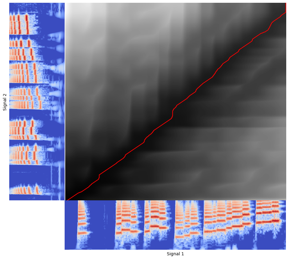
Visualize both signals and their alignment:
plt.figure(figsize=(9, 8))

# Bottom right plot.
ax1 = plt.axes([0.2, 0, 0.8, 0.20])
ax1.imshow(C1_cqt_mag, origin="lower", aspect="auto", cmap="coolwarm")
ax1.set_xlabel("Signal 1")
ax1.set_xticks([])
ax1.set_yticks([])
ax1.set_ylim(20)

# Top left plot.
ax2 = plt.axes([0, 0.2, 0.20, 0.8])
ax2.imshow(C2_cqt_mag.T[:, ::-1], origin="lower", aspect="auto", cmap="coolwarm")
ax2.set_ylabel("Signal 2")
ax2.set_xticks([])
ax2.set_yticks([])
ax2.set_ylim(20)

# Top right plot.
ax3 = plt.axes([0.2, 0.2, 0.8, 0.8], sharex=ax1, sharey=ax2)
ax3.imshow(D.T, aspect="auto", origin="lower", interpolation="nearest", cmap="gray")
ax3.set_xticks([])
ax3.set_yticks([])

# Path.
ax3.plot(path[:, 0], path[:, 1], "r")
[<matplotlib.lines.Line2D at 0x711bd6adab30>]
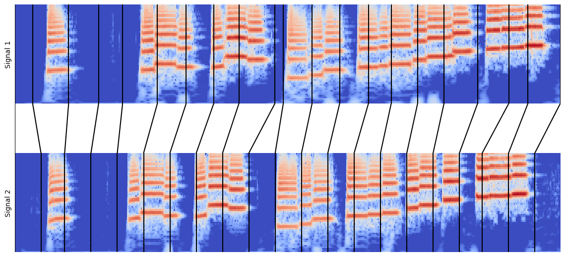
plt.figure(figsize=(11, 5))

# Top plot.
ax1 = plt.axes([0, 0.60, 1, 0.40])
ax1.imshow(C1_cqt_mag, origin="lower", aspect="auto", cmap="coolwarm")
ax1.set_ylabel("Signal 1")
ax1.set_xticks([])
ax1.set_yticks([])
ax1.set_ylim(20)
ax1.set_xlim(0, C1_cqt.shape[1])

# Bottom plot.
ax2 = plt.axes([0, 0, 1, 0.40])
ax2.imshow(C2_cqt_mag, origin="lower", aspect="auto", cmap="coolwarm")
ax2.set_ylabel("Signal 2")
ax2.set_xticks([])
ax2.set_yticks([])
ax2.set_ylim(20)
ax2.set_xlim(0, C2_cqt.shape[1])

# Middle plot.
line_color = "k"
step = 30
n1 = float(C1_cqt.shape[1])
n2 = float(C2_cqt.shape[1])
ax3 = plt.axes([0, 0.40, 1, 0.20])
for t in path[::step]:
    ax3.plot((t[0] / n1, t[1] / n2), (1, -1), color=line_color)
    ax3.set_xlim(0, 1)
    ax3.set_ylim(-1, 1)

# Path markers on top and bottom plot.
y1_min, y1_max = ax1.get_ylim()
y2_min, y2_max = ax2.get_ylim()
ax1.vlines([t[0] for t in path[::step]], y1_min, y1_max, color=line_color)
ax2.vlines([t[1] for t in path[::step]], y2_min, y2_max, color=line_color)
ax3.set_xticks([])
ax3.set_yticks([])
[]
Exercises#
Try each pair of audio files among the following:
mirdotcom.list_audio("sir_duke")
assets/audio/sir_duke_piano_fast.mp3  assets/audio/sir_duke_trumpet_fast.mp3
assets/audio/sir_duke_piano_slow.mp3  assets/audio/sir_duke_trumpet_slow.mp3
Try adjusting the hop length, distance metric, and feature space.
Instead of chroma_cens, try chroma_stft or librosa.feature.mfcc.
Try magnitude scaling the feature matrices, e.g. amplitude_to_db or \(\log(1 + \lambda x)\).