Jupyter Audio Basics#
from mirdotcom import mirdotcom

mirdotcom.init()
Audio Libraries#
We will mainly use two libraries for audio acquisition and playback:
1. librosa#
librosa is a Python package for music and audio processing by Brian McFee. A large portion was ported from Dan Ellis’s Matlab audio processing examples.
2. IPython.display.Audio#
IPython.display.Audio lets you play audio directly in an IPython notebook.
Included Audio Data#
This GitHub repository includes many short audio excerpts for your convenience.
Here are the files currently in the audio directory:
mirdotcom.list_audio()
simple_piano.wav
latin_groove.mp3
clarinet_c6.wav
cowbell.wav
classic_rock_beat.mp3
oboe_c6.wav
sir_duke_trumpet_fast.mp3
sir_duke_trumpet_slow.mp3
jangle_pop.mp3
125_bounce.wav
brahms_hungarian_dance_5.mp3
58bpm.wav
conga_groove.wav
funk_groove.mp3
tone_440.wav
sir_duke_piano_fast.mp3
thx_original.mp3
simple_loop.wav
classic_rock_beat.wav
c_strum.wav
prelude_cmaj.wav
sir_duke_piano_slow.mp3
busta_rhymes_hits_for_days.mp3
Visit https://ccrma.stanford.edu/workshops/mir2014/audio/ for more audio files.
Reading Audio#
Use librosa.load to load an audio file into an audio array. Return both the audio array as well as the sample rate:
import librosa

fp = mirdotcom.get_audio("simple_loop.wav")
x, sr = librosa.load(fp)
If you receive an error with librosa.load, you may need to install ffmpeg.
Display the length of the audio array and sample rate:
print(x.shape)
print(sr)
(49613,)
22050
Visualizing Audio#
In order to display plots inside the Jupyter notebook, run the following commands, preferably at the top of your notebook:
%matplotlib inline
import matplotlib.pyplot as plt
import librosa.display
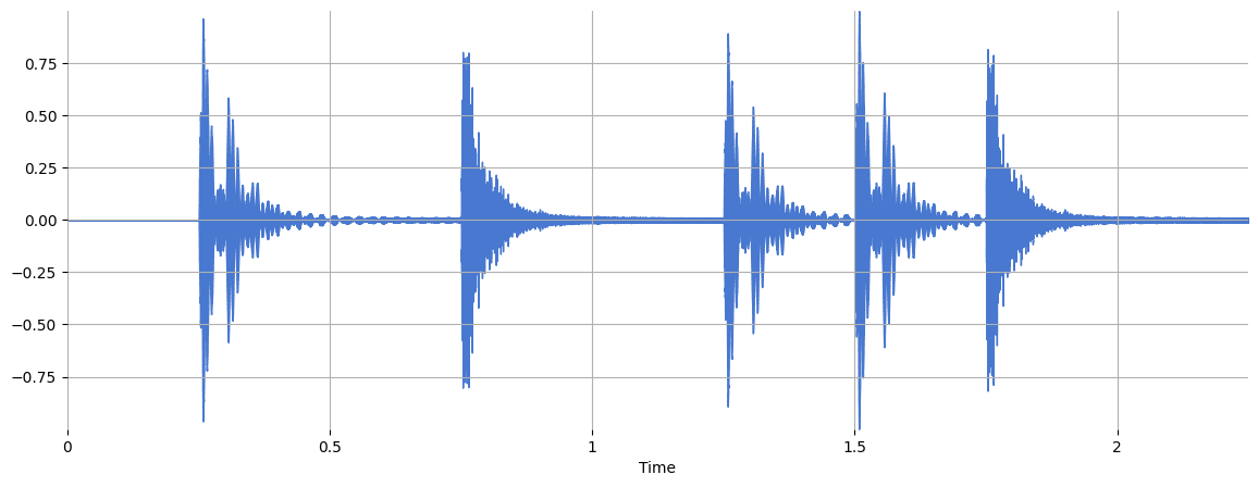
Plot the audio array using librosa.display.waveshow:
plt.figure(figsize=(14, 5))
librosa.display.waveshow(x, sr=sr)
<librosa.display.AdaptiveWaveplot at 0x7df465c59810>
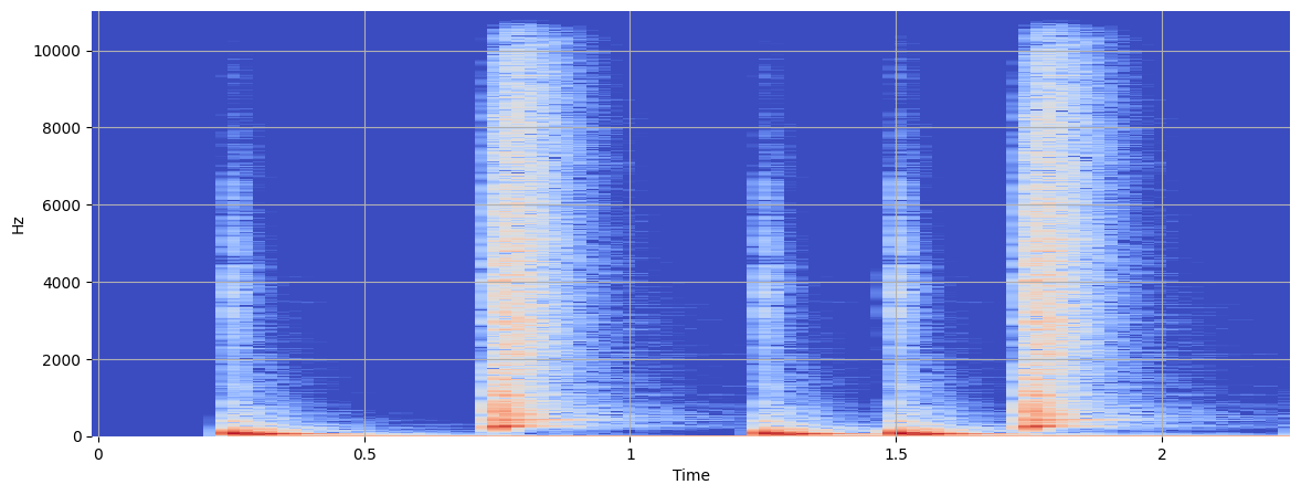
Display a spectrogram using librosa.display.specshow:
X = librosa.stft(x)
Xdb = librosa.amplitude_to_db(abs(X))
plt.figure(figsize=(14, 5))
librosa.display.specshow(Xdb, sr=sr, x_axis="time", y_axis="hz")
<matplotlib.collections.QuadMesh at 0x7df4657620e0>
Playing Audio#
IPython.display.Audio#
Using IPython.display.Audio, you can play an audio file:
import IPython.display as ipd

fp = mirdotcom.get_audio("conga_groove.wav")
ipd.Audio(fp)  # load a local WAV file
Audio can also accept a NumPy array. Let’s synthesize a pure tone at 440 Hz:
import numpy

sr = 22050  # sample rate
T = 2.0  # seconds
t = numpy.linspace(0, T, int(T * sr), endpoint=False)  # time variable
x = 0.5 * numpy.sin(2 * numpy.pi * 440 * t)  # pure sine wave at 440 Hz
Listen to the audio array:
ipd.Audio(x, rate=sr) # load a NumPy array
Writing Audio#
soundfile.write saves a NumPy array to a WAV file.
import soundfile

fp = mirdotcom.get_audio("tone_440.wav")
soundfile.write(fp, x, sr)