Magnitude Scaling#
import warnings

import IPython.display as ipd
import matplotlib.pyplot as plt
import librosa.display
import numpy

from mirdotcom import mirdotcom

warnings.filterwarnings("ignore")
mirdotcom.init()
Often, the raw amplitude of a signal in the time- or frequency-domain is not as perceptually relevant to humans as the amplitude converted into other units, e.g. using a logarithmic scale.
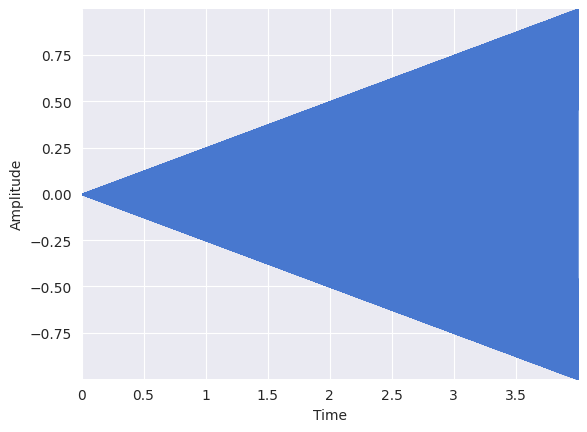
For example, let’s consider a pure tone whose amplitude grows louder linearly. Define the time variable:
T = 4.0  # duration in seconds
sr = 22050  # sampling rate in Hertz
t = numpy.linspace(0, T, int(T * sr), endpoint=False)
Create a signal whose amplitude grows linearly:
amplitude = numpy.linspace(0, 1, int(T * sr), endpoint=False)  # time-varying amplitude
x = amplitude * numpy.sin(2 * numpy.pi * 440 * t)
Listen:
ipd.Audio(x, rate=sr)
Plot the signal:
librosa.display.waveshow(x, sr=sr)
plt.ylabel("Amplitude")
Text(22.472222222222214, 0.5, 'Amplitude')
Now consider a signal whose amplitude grows exponentially, i.e. the logarithm of the amplitude is linear:
amplitude = numpy.logspace(-2, 0, int(T * sr), endpoint=False, base=10.0)
x = amplitude * numpy.sin(2 * numpy.pi * 440 * t)
ipd.Audio(x, rate=sr)
librosa.display.waveshow(x, sr=sr)
plt.ylabel("Amplitude")
Text(22.472222222222214, 0.5, 'Amplitude')
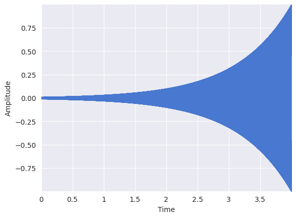
Even though the amplitude grows exponentially, to us, the increase in loudness seems more gradual. This phenomenon is an example of the Weber-Fechner law (Wikipedia) which states that the relationship between a stimulus and human perception is logarithmic.
Spectrogram Visualization: Linear Amplitude#
Let’s plot a magnitude spectrogram where the colorbar is a linear function of the spectrogram values, i.e. just plot the raw values.
fp = mirdotcom.get_audio("latin_groove.mp3")
x, sr = librosa.load(fp, duration=8)
ipd.Audio(x, rate=sr)
X = librosa.stft(x)
X.shape
(1025, 345)
Raw amplitude:
Xmag = abs(X)
librosa.display.specshow(Xmag, sr=sr, x_axis="time", y_axis="log")
plt.colorbar()
<matplotlib.colorbar.Colorbar at 0x7091ad41ad10>
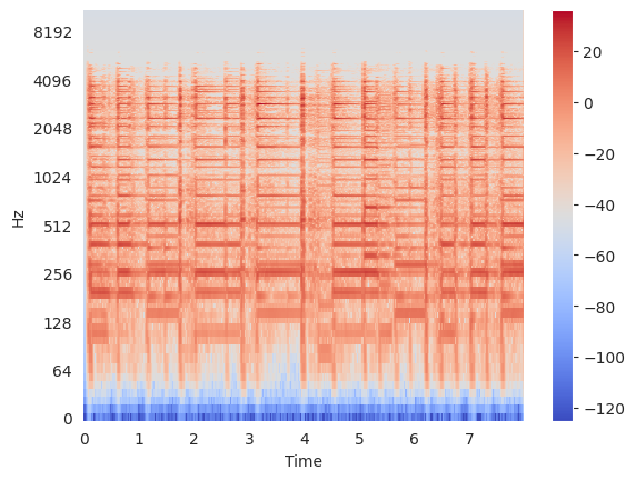
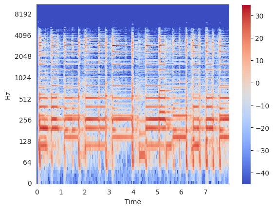
Spectrogram Visualization: Log Amplitude#
Now let’s plot a magnitude spectrogram where the colorbar is a logarithmic function of the spectrogram values.
Decibel (Wikipedia)
Xdb = librosa.amplitude_to_db(Xmag)
librosa.display.specshow(Xdb, sr=sr, x_axis="time", y_axis="log")
plt.colorbar()
<matplotlib.colorbar.Colorbar at 0x7091ad312950>
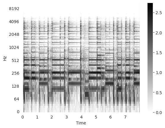
One common variant is the \(\log (1 + \lambda x)\) function, sometimes known as logarithmic compression (FMP, p. 125). This function operates like \(y = \lambda x\) when \(\lambda x\) is small, but it operates like \(y = \log \lambda x\) when \(\lambda x\) is large.
Xmag = numpy.log10(1 + 10 * abs(X))
librosa.display.specshow(Xmag, sr=sr, x_axis="time", y_axis="log", cmap="gray_r")
plt.colorbar()
<matplotlib.colorbar.Colorbar at 0x7091ad2241f0>
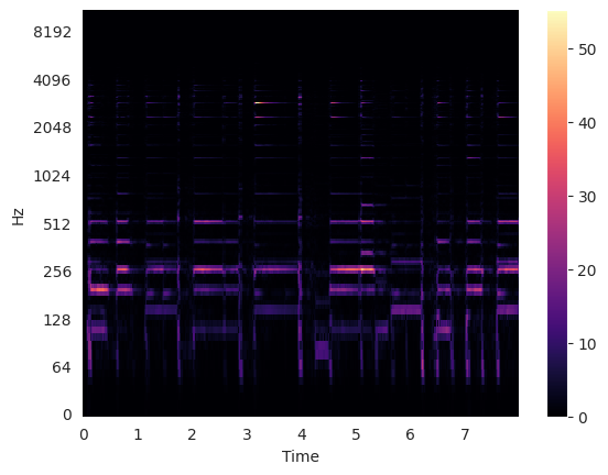
Spectrogram Visualization: Perceptual Weighting#
freqs = librosa.core.fft_frequencies(sr=sr)
Xmag = librosa.perceptual_weighting(abs(X) ** 2, freqs)
librosa.display.specshow(Xmag, sr=sr, x_axis="time", y_axis="log")
plt.colorbar()
<matplotlib.colorbar.Colorbar at 0x7091ad1060b0>