THX Logo Theme

THX Logo Theme#

import IPython.display as ipd
import matplotlib.pyplot as plt
import librosa.display
import numpy

from mirdotcom import mirdotcom

mirdotcom.init()

What is the THX logo theme?#

THX posted the score of the original THX logo theme on Twitter:

%%html
<blockquote class="twitter-tweet" data-lang="en"><p lang="en" dir="ltr">In 35 yrs we have NEVER shown this! View the never-before-seen score of <a href="https://twitter.com/hashtag/DeepNote?src=hash&amp;ref_src=twsrc%5Etfw">#DeepNote</a> THX&#39;s audio trademark 🔊 created by Dr. James A. Moorer a former employee of <a href="https://twitter.com/hashtag/Lucasfilm?src=hash&amp;ref_src=twsrc%5Etfw">#Lucasfilm</a>. <a href="https://twitter.com/hashtag/DeepNote?src=hash&amp;ref_src=twsrc%5Etfw">#DeepNote</a> debuted at the premiere of <a href="https://twitter.com/hashtag/ReturnOfTheJedi?src=hash&amp;ref_src=twsrc%5Etfw">#ReturnOfTheJedi</a> on May 25th 1983 // 35yrs ago <a href="https://twitter.com/hashtag/THXLtdEntertainsAt35?src=hash&amp;ref_src=twsrc%5Etfw">#THXLtdEntertainsAt35</a> <a href="https://twitter.com/hashtag/RT?src=hash&amp;ref_src=twsrc%5Etfw">#RT</a> <a href="https://t.co/9LLF6Ul17m">https://pic.twitter.com/9LLF6Ul17m</a></p>&mdash; THX Ltd. (@THX) <a href="https://twitter.com/THX/status/1000077588415447040?ref_src=twsrc%5Etfw">May 25, 2018</a></blockquote>
<script async src="https://platform.twitter.com/widgets.js" charset="utf-8"></script>

In 35 yrs we have NEVER shown this! View the never-before-seen score of #DeepNote THX's audio trademark 🔊 created by Dr. James A. Moorer a former employee of #Lucasfilm. #DeepNote debuted at the premiere of #ReturnOfTheJedi on May 25th 1983 // 35yrs ago #THXLtdEntertainsAt35 #RT pic.twitter.com/9LLF6Ul17m
— THX Ltd. (@THX) May 25, 2018

If you’re not familiar, here is the trademark sound:

ipd.YouTubeVideo("6grjzBmHVTY", start=10, end=26)

Following the instructions in the score, here is a simpler version of the THX logo theme. It may not be exactly the same, but it comes close.

Signal Model#

For voice \(i\), we have the following sinusoid with a time-dependent amplitude and frequency:

\[ x_i(t) = A(t) \sin(2 \pi f_i(t) t) \]

The output is a sum of the voices:

\[ y(t) = \sum_i x_i(t) = A(t) \sum_i \sin(2 \pi f_i(t) t) \]

In discrete time, for sampling rate/frequency \(f_s\),

\[ y[n] = \sum_i x_i[n] = A[n] \sum_i \sin(2 \pi f_i[n] n/f_s) \]

Stages#

We define four stages in the signal:

During the start, voice frequencies move randomly within a narrow frequency range, and voices are quiet.
During the transition, voices move toward their target frequency, and voices become louder.
During the sustain, voices remain at their target frequency, and voices are loud.
During the decay, voices become quieter.

Here are the times when the start, transition, sustain, and decay stages begin. t_end is the end of the signal.

t_start = 0
t_transition = 4
t_sustain = 10
t_decay = 14
t_end = 16

Define a sample rate:

sr = 44100

Convert these times to units of samples:

n_start = t_start * sr
n_transition = t_transition * sr
n_sustain = t_sustain * sr
n_decay = t_decay * sr
n_end = t_end * sr

Define time axis in units of samples and seconds:

n = numpy.arange(n_end)
t = n / sr

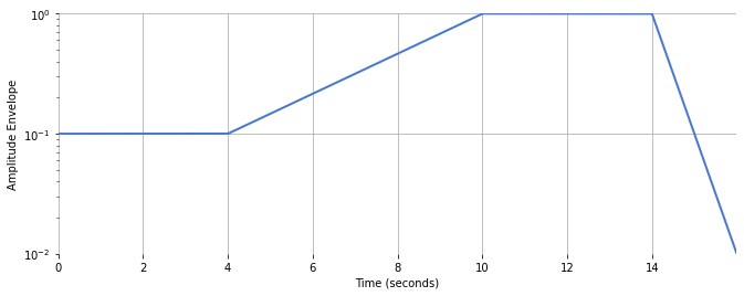
Amplitude#

For each of the four stages above, define amplitude envelope, \(A(t)\).

The start stage, sustain stage, and end will have constant amplitudes:

amplitude_start = 0.1
amplitude_sustain = 1
amplitude_end = 0.01

The transition and decay stages will increase or decrease following a geometric/exponential sequence:

amplitude_transition = numpy.geomspace(
    amplitude_start, amplitude_sustain, n_sustain - n_transition
)
amplitude_decay = numpy.geomspace(amplitude_sustain, amplitude_end, n_end - n_decay)

Create the amplitude envelope:

amplitude = numpy.zeros(n_end)
amplitude[n_start:n_transition] = amplitude_start
amplitude[n_transition:n_sustain] = amplitude_transition
amplitude[n_sustain:n_decay] = amplitude_sustain
amplitude[n_decay:n_end] = amplitude_decay

Plot amplitude envelope with a log-y axis:

plt.figure(figsize=(11, 4))
plt.semilogy(t, amplitude, linewidth=2)
plt.xlabel("Time (seconds)")
plt.ylabel("Amplitude Envelope")

Text(0, 0.5, 'Amplitude Envelope')

Frequency#

Revisiting the model above, for voice \(i\),

\[ x_i[n] \propto \sin(2 \pi f_i[n] n/f_s) \]

Define \(\phi_i[n] = f_i[n] n\). Therefore, \( x_i[n] \propto \sin((2 \pi/f_s) \phi_i[n] ) \).

Suppose \(f_i\) remains constant over time. Then we have the following update rule:

\[ \phi[n] - \phi[n-1] = f_i n - f_i(n-1) = f_i \]

\[ \Rightarrow \phi[n] = \phi[n-1] + f_i \]

Now suppose \(f_i[n]\) changes over time. Then we can simply use the following update rule instead:

\[ \phi[n] = \phi[n-1] + f_i[n] \]

This update rule is simply a cumulative sum of \(f_i[n]\)!

Let’s define the frequencies during the final sustain phase, i.e. the final four measures. We tune the concert-A to be 448 Hz which seems to match the original recording. Then we simply define notes at A and D at different octaves. We use Pythagorean tuning, i.e. perfect fifths have a frequency ratio of 3:2, and octaves have a frequency ratio of 2:1.

f_sustain = [
    448 * x
    for x in [
        1 / 12,
        1 / 8,
        1 / 6,
        1 / 4,
        1 / 3,
        1 / 2,
        2 / 3,
        1,
        4 / 3,
        2,
        8 / 3,
        4,
        16 / 3,
        8,
    ]
] * 3

Total number of voices:

num_voices = len(f_sustain)
num_voices

Then, we create our time-dependent frequecies for each voice.

fmin = librosa.note_to_hz("C0")
fmax = librosa.note_to_hz("C9")
n_bins = 9 * 12  # 9 octaves

phi = [None] * num_voices
f_lo = librosa.note_to_hz("C3")
plt.figure(figsize=(15, 9))

for voice in range(num_voices):

    # Initialize frequency array.
    f = numpy.zeros(n_end)

    # Initial frequencies are random between C3 and C5.
    f1 = f_lo * 4 ** numpy.random.rand()
    f2 = f_lo * 4 ** numpy.random.rand()
    f_transition = f_lo * 4 ** numpy.random.rand()

    # Define one random time point during the start stage.
    n1 = numpy.random.randint(n_start, n_transition)

    # Assign frequencies to each stage.
    f[n_start:n1] = numpy.geomspace(f1, f2, n1 - n_start)
    f[n1:n_transition] = numpy.geomspace(f2, f_transition, n_transition - n1)
    f[n_transition:n_sustain] = numpy.geomspace(
        f_transition, f_sustain[voice], n_sustain - n_transition
    )
    f[n_sustain:n_end] = f_sustain[voice]

    # Perform the update rule. Easy!
    phi[voice] = numpy.cumsum(f)

    # Plot frequency.
    plt.semilogy(t, f)

plt.xlabel("Time (seconds)")
plt.ylabel("Frequency (Hertz)")
plt.ylim(fmin, fmax)

(16.351597831287414, 8372.018089619156)

Synthesize output#

Initialize the output signal:

out_signal = numpy.zeros(n_end)

Finally, construct the output signal, one voice at a time:

for voice in range(num_voices):
    out_signal += numpy.sin(2 * numpy.pi / sr * phi[voice])

Normalize the signal amplitude:

out_signal *= amplitude
out_signal *= 0.99 / out_signal.max()

Listen:

ipd.Audio(out_signal, rate=sr)

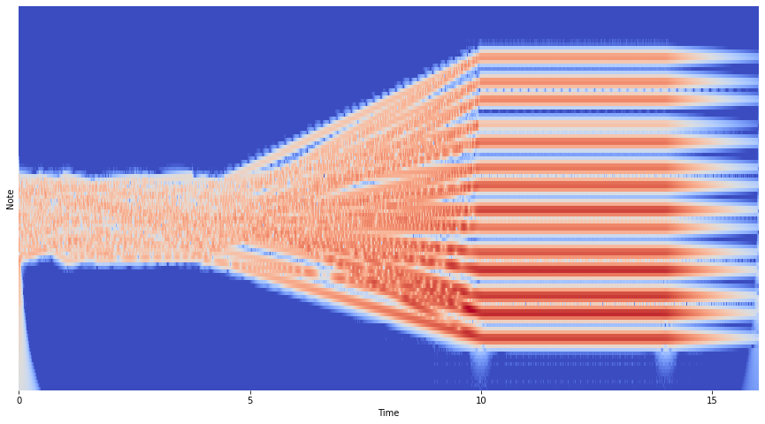
Pretty cool!

C = librosa.cqt(out_signal, sr=sr, fmin=fmin, n_bins=n_bins)
C_db = librosa.amplitude_to_db(abs(C))
plt.figure(figsize=(15, 8))
librosa.display.specshow(
    C_db, sr=sr, x_axis="time", y_axis="cqt_note", fmin=fmin, cmap="coolwarm"
)

<matplotlib.collections.QuadMesh at 0x7f091e873c10>

How does it compare to the original?#

filename = mirdotcom.get_audio("thx_original.mp3")
thx, sr_thx = librosa.load(filename)

/usr/local/lib/python3.7/dist-packages/librosa/core/audio.py:165: UserWarning: PySoundFile failed. Trying audioread instead.
  warnings.warn("PySoundFile failed. Trying audioread instead.")

ipd.Audio(thx, rate=sr_thx)

C = librosa.cqt(thx, sr=sr_thx, fmin=fmin, n_bins=n_bins)

C_db = librosa.amplitude_to_db(abs(C))
plt.figure(figsize=(15, 8))
librosa.display.specshow(
    C_db, sr=sr_thx, x_axis="time", y_axis="cqt_note", fmin=fmin, cmap="coolwarm"
)