Spectral Features

import IPython.display as ipd
import matplotlib.pyplot as plt
import librosa.display
import sklearn

from mirdotcom import mirdotcom

mirdotcom.init()

For classification, we’re going to be using new features in our arsenal: spectral moments (centroid, bandwidth, skewness, kurtosis) and other spectral statistics.

A moment is a term used in physics and statistics. There are raw moments and central moments.

You are probably already familiar with two examples of moments: mean and variance. The first raw moment is known as the mean. The second central moment is known as the variance.

Spectral Centroid

Load an audio file:

filename = mirdotcom.get_audio("simple_loop.wav")
x, sr = librosa.load(filename)
ipd.Audio(x, rate=sr)

The spectral centroid (Wikipedia) indicates at which frequency the energy of a spectrum is centered upon. This is like a weighted mean:

\[ f_c = \frac{\sum_k S(k) f(k)}{\sum_k S(k)} \]

where \(S(k)\) is the spectral magnitude at frequency bin \(k\), \(f(k)\) is the frequency at bin \(k\).

librosa.feature.spectral_centroid computes the spectral centroid for each frame in a signal:

spectral_centroids = librosa.feature.spectral_centroid(y=x, sr=sr)[0]
spectral_centroids.shape

(97,)

Compute the time variable for visualization:

frames = range(len(spectral_centroids))
t = librosa.frames_to_time(frames)

Define a helper function to normalize the spectral centroid for visualization:

def normalize(x, axis=0):
    return sklearn.preprocessing.minmax_scale(x, axis=axis)

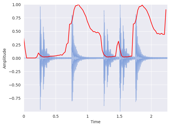
Plot the spectral centroid along with the waveform:

librosa.display.waveshow(x, sr=sr, alpha=0.4)
plt.plot(
    t, normalize(spectral_centroids), color="r"
)  # normalize for visualization purposes
plt.ylabel("Amplitude")

Text(22.472222222222214, 0.5, 'Amplitude')

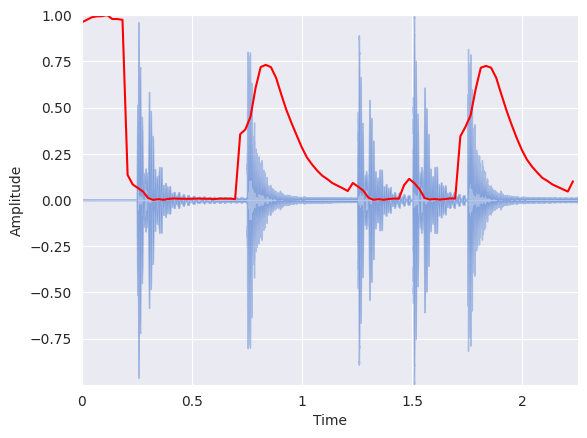
Similar to the zero crossing rate, there is a spurious rise in spectral centroid at the beginning of the signal. That is because the silence at the beginning has such small amplitude that high frequency components have a chance to dominate. One hack around this is to add a small constant before computing the spectral centroid, thus shifting the centroid toward zero at quiet portions:

spectral_centroids = librosa.feature.spectral_centroid(y=x + 0.01, sr=sr)[0]
librosa.display.waveshow(x, sr=sr, alpha=0.4)
plt.plot(
    t, normalize(spectral_centroids), color="r"
)  # normalize for visualization purposes
plt.ylabel("Amplitude")

Text(22.472222222222214, 0.5, 'Amplitude')

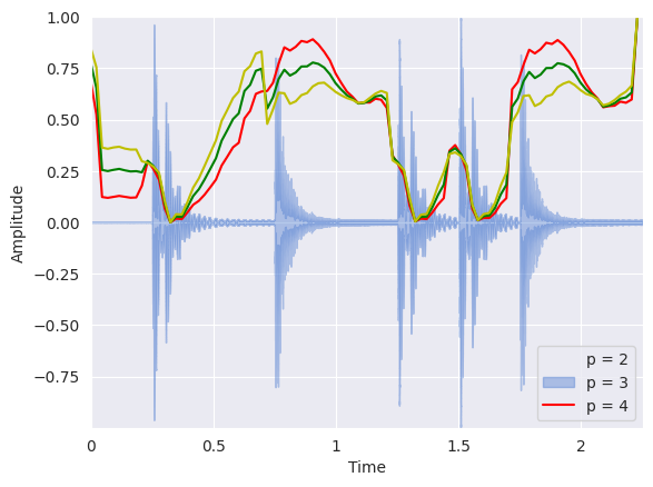
Spectral Bandwidth

librosa.feature.spectral_bandwidth computes the order-\(p\) spectral bandwidth:

\[ \left( \sum_k S(k) \left(f(k) - f_c \right)^p \right)^{\frac{1}{p}} \]

where \(S(k)\) is the spectral magnitude at frequency bin \(k\), \(f(k)\) is the frequency at bin \(k\), and \(f_c\) is the spectral centroid. When \(p = 2\), this is like a weighted standard deviation.

spectral_bandwidth_2 = librosa.feature.spectral_bandwidth(y=x + 0.01, sr=sr)[0]
spectral_bandwidth_3 = librosa.feature.spectral_bandwidth(y=x + 0.01, sr=sr, p=3)[0]
spectral_bandwidth_4 = librosa.feature.spectral_bandwidth(y=x + 0.01, sr=sr, p=4)[0]
librosa.display.waveshow(x, sr=sr, alpha=0.4)
plt.plot(t, normalize(spectral_bandwidth_2), color="r")
plt.plot(t, normalize(spectral_bandwidth_3), color="g")
plt.plot(t, normalize(spectral_bandwidth_4), color="y")
plt.legend(("p = 2", "p = 3", "p = 4"))
plt.ylabel("Amplitude")

Text(22.472222222222214, 0.5, 'Amplitude')

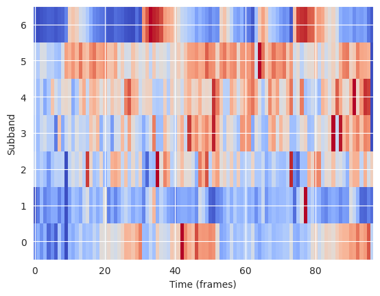
Spectral Contrast

Spectral contrast considers the spectral peak, the spectral valley, and their difference in each frequency subband. For more information:

• Jiang, Dan-Ning, Lie Lu, Hong-Jiang Zhang, Jian-Hua Tao, and Lian-Hong Cai. “Music type classification by spectral contrast feature.” In Multimedia and Expo, 2002. ICME‘02. Proceedings. 2002 IEEE International Conference on, vol. 1, pp. 113-116. IEEE, 2002.

librosa.feature.spectral_contrast computes the spectral contrast for six subbands for each time frame:

spectral_contrast = librosa.feature.spectral_contrast(y=x, sr=sr)
spectral_contrast.shape

(7, 97)

Display:

plt.imshow(
    normalize(spectral_contrast, axis=1), aspect="auto", origin="lower", cmap="coolwarm"
)
plt.ylabel("Subband")
plt.xlabel("Time (frames)")

Text(0.5, 0, 'Time (frames)')

Spectral Rolloff

Spectral rolloff is the frequency below which a specified percentage of the total spectral energy, e.g. 85%, lies.

librosa.feature.spectral_rolloff computes the rolloff frequency for each frame in a signal:

spectral_rolloff = librosa.feature.spectral_rolloff(y=x + 0.01, sr=sr)[0]
librosa.display.waveshow(x, sr=sr, alpha=0.4)
plt.plot(t, normalize(spectral_rolloff), color="r")
plt.ylabel("Amplitude")

Text(22.472222222222214, 0.5, 'Amplitude')