NMF Audio Mosaicing

import IPython.display as ipd
import matplotlib.pyplot as plt
import librosa.display
import numpy

from mirdotcom import mirdotcom

mirdotcom.init()

This notebook is inspired by the work of Jonathan Driedger, Thomas Prätzlich, and Meinard Müller.

Here is a fun exercise to understand how NMF works. We are going to synthesize an audio signal, \(y\), using spectral content from one audio signal, \(x_1\), and the NMF temporal activations from another audio signal, \(x_2\).

Step 1: Compute the STFT of the first signal, \(x_1\):

\[ X_1 \leftarrow \textrm{STFT}(x_1) \]

Step 2: Perform NMF on the second signal, \(x_2\), to learn temporal activations while fixing the spectral profiles to the magnitude spectrogram, \(|X_1|\), learned in step 1:

\[ H \leftarrow \textrm{NMF}(x_2, |X_1|) \]

Step 3: Synthesize an audio signal using \(|X_1|\) and \(H\):

\[ y \leftarrow \textrm{ISTFT}(|X_1| H) \]

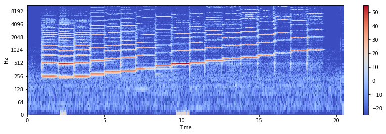
Step 1: Magnitude Spectrogram of Signal 1

Load the first signal, \(x_1\):

filename = mirdotcom.get_audio("oboe_c6.wav")
x1, sr = librosa.load(filename)

ipd.Audio(x1, rate=sr)

Compute STFT \(X_1\), and separate into magnitude and phase:

X1 = librosa.stft(x1)
X1_mag, X1_phase = librosa.magphase(X1)

X1_db = librosa.amplitude_to_db(X1_mag)
plt.figure(figsize=(14, 4))
librosa.display.specshow(X1_db, sr=sr, x_axis="time", y_axis="log")
plt.colorbar()

<matplotlib.colorbar.Colorbar at 0x1116d7828>

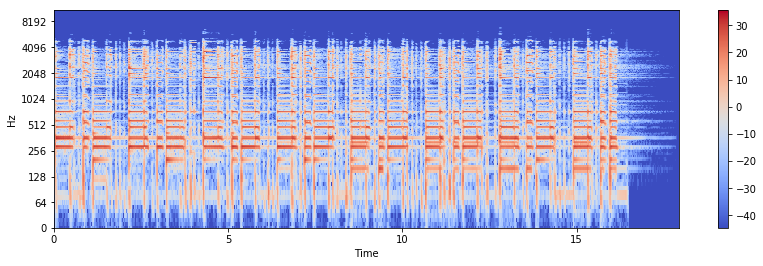
Step 2: NMF on Signal 2

Load the second signal, \(x_2\):

filename = mirdotcom.get_audio("funk_groove.mp3")
x2, _ = librosa.load(filename)

ipd.Audio(x2, rate=sr)

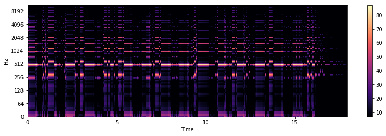
Compute STFT \(X_2\), and separate into magnitude and phase:

X2 = librosa.stft(x2)
X2_mag, X2_phase = librosa.magphase(X2)

X2_db = librosa.amplitude_to_db(X2_mag)
plt.figure(figsize=(14, 4))
librosa.display.specshow(X2_db, sr=sr, x_axis="time", y_axis="log")
plt.colorbar()

<matplotlib.colorbar.Colorbar at 0x11603f2e8>

Define \(W \triangleq |X_1|\). \(W\) will remain fixed.

Perform NMF, but we will only apply an update to \(H\), not \(W\):

\[ H \leftarrow H \frac{W^T |X_2|}{W^T W H} \]

For this, we will write our own multiplicative update rule that only updates \(H\):

# Cache some matrix multiplications.
W = librosa.util.normalize(X1_mag, norm=2, axis=0)
WTX = W.T.dot(X2_mag)
WTW = W.T.dot(W)

# Initialize H.
H = numpy.random.rand(X1.shape[1], X2.shape[1])

# Update H.
eps = 0.01
for _ in range(100):
    H = H * (WTX + eps) / (WTW.dot(H) + eps)

H.shape

(881, 772)

plt.imshow(H.T.dot(H))

<matplotlib.image.AxesImage at 0x108a6afd0>

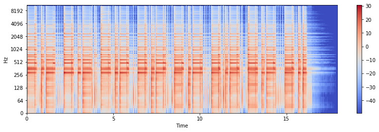
Step 3: Synthesize Output Signal

Synthesize the output signal, \(y\), from the spectral components of \(x_1\) and the temporal activations (and phase) of \(x_2\):

Y_mag = W.dot(H)

Y_db = librosa.amplitude_to_db(Y_mag)
plt.figure(figsize=(14, 4))
librosa.display.specshow(Y_db, sr=sr, x_axis="time", y_axis="log")
plt.colorbar()

<matplotlib.colorbar.Colorbar at 0x1112cc0f0>

Y = Y_mag * X2_phase
y = librosa.istft(Y)

ipd.Audio(y, rate=sr)

Alternate Approach: Sparse Coding

from sklearn.decomposition import SparseCoder

sparse_coder = SparseCoder(X1_mag.T, transform_n_nonzero_coefs=1)

H = sparse_coder.transform(X2_mag.T)

H.shape

(772, 881)

plt.imshow(H.T.dot(H))

<matplotlib.image.AxesImage at 0x1160d4320>

Y_mag = W.dot(H.T)

Y_db = librosa.amplitude_to_db(Y_mag)
plt.figure(figsize=(14, 4))
librosa.display.specshow(Y_db, sr=sr, x_axis="time", y_axis="log")
plt.colorbar()

<matplotlib.colorbar.Colorbar at 0x115fd4518>

Y = Y_mag * X2_phase
y = librosa.istft(Y)

ipd.Audio(y, rate=sr)