Harmonic-Percussive Source Separation

import IPython.display as ipd
import matplotlib.pyplot as plt
import librosa.display

from mirdotcom import mirdotcom

mirdotcom.init()

Load two files: one harmonic, and one percussive.

filename = mirdotcom.get_audio("prelude_cmaj.wav")
xh, sr_h = librosa.load(filename, duration=7, sr=None)

ipd.Audio(xh, rate=sr_h)

filename = mirdotcom.get_audio("125_bounce.wav")
xp, sr_p = librosa.load(filename, duration=7, sr=None)

ipd.Audio(xp, rate=sr_p)

print(len(xh), len(xp))

154350 154350

print(sr_h, sr_p)

22050 22050

Add the two signals together, and rescale:

x = xh / xh.max() + xp / xp.max()
x = 0.5 * x / x.max()

x.max()

0.5

Listen to the combined audio signal:

ipd.Audio(x, rate=sr_h)

Compute the STFT:

X = librosa.stft(x)

Take the log-ampllitude for display purposes:

Xmag = librosa.amplitude_to_db(X)

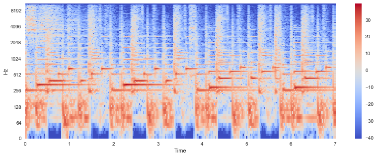
Display the log-magnitude spectrogram:

librosa.display.specshow(Xmag, sr=sr_h, x_axis="time", y_axis="log")
plt.colorbar()

<matplotlib.colorbar.Colorbar at 0x1139b14d0>

Perform harmonic-percussive source separation:

H, P = librosa.decompose.hpss(X)

Compute the log-amplitudes of the outputs:

Hmag = librosa.amplitude_to_db(H)
Pmag = librosa.amplitude_to_db(P)

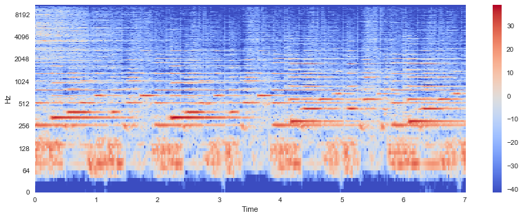
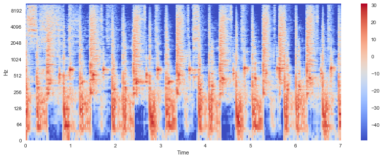
Display each output:

librosa.display.specshow(Hmag, sr=sr_h, x_axis="time", y_axis="log")
plt.colorbar()

<matplotlib.colorbar.Colorbar at 0x1139c2410>

librosa.display.specshow(Pmag, sr=sr_p, x_axis="time", y_axis="log")
plt.colorbar()

<matplotlib.colorbar.Colorbar at 0x1134df950>

Transform the harmonic output back to the time domain:

h = librosa.istft(H)

Listen to the harmonic output:

ipd.Audio(h, rate=sr_h)

Transform the percussive output back to the time domain:

p = librosa.istft(P)

Listen to the percussive output:

ipd.Audio(p, rate=sr_p)