Autocorrelation

The autocorrelation of a signal describes the similarity of a signal against a time-shifted version of itself. For a signal \(x\), the autocorrelation \(r\) is:

\[ r(k) = \sum_n x(n) x(n-k) \]

In this equation, \(k\) is often called the lag parameter. \(r(k)\) is maximized at \(k = 0\) and is symmetric about \(k\).

The autocorrelation is useful for finding repeated patterns in a signal. For example, at short lags, the autocorrelation can tell us something about the signal’s fundamental frequency. For longer lags, the autocorrelation may tell us something about the tempo of a musical signal.

import IPython.display as ipd
import matplotlib.pyplot as plt
import librosa.display
import numpy

from mirdotcom import mirdotcom

mirdotcom.init()

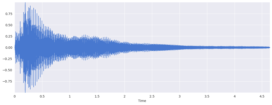
Let’s load a file:

fp = mirdotcom.get_audio("c_strum.wav")
x, sr = librosa.load(fp)
ipd.Audio(x, rate=sr)

plt.figure(figsize=(14, 5))
librosa.display.waveshow(x, sr=sr)

<librosa.display.AdaptiveWaveplot at 0x743b257d6c20>

Using numpy

There are two ways we can compute the autocorrelation in Python. The first method is numpy.correlate:

# Because the autocorrelation produces a symmetric signal, we only care about the "right half".
r = numpy.correlate(x, x, mode="full")[len(x) - 1 :]
print(x.shape, r.shape)

(102400,) (102400,)

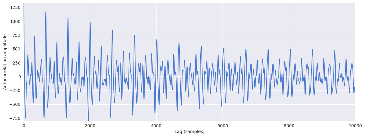
Plot the autocorrelation:

plt.figure(figsize=(14, 5))
plt.plot(r[:10000])
plt.xlabel("Lag (samples)")
plt.ylabel("Autocorrelation amplitude")
plt.xlim(0, 10000)

(0.0, 10000.0)

Using librosa

The second method is librosa.autocorrelate:

r = librosa.autocorrelate(x, max_size=10000)
print(r.shape)

(10000,)

plt.figure(figsize=(14, 5))
plt.plot(r)
plt.xlabel("Lag (samples)")
plt.ylabel("Autocorrelation amplitude")
plt.xlim(0, 10000)

(0.0, 10000.0)

librosa.autocorrelate conveniently only keeps one half of the autocorrelation function, since the autocorrelation is symmetric. Also, the max_size parameter prevents unnecessary calculations.

Pitch Estimation

The autocorrelation is used to find repeated patterns within a signal. For musical signals, a repeated pattern can correspond to a pitch period. We can therefore use the autocorrelation function to estimate the pitch in a musical signal.

fp = mirdotcom.get_audio("oboe_c6.wav")
x, sr = librosa.load(fp)
ipd.Audio(x, rate=sr)

Compute and plot the autocorrelation:

r = librosa.autocorrelate(x, max_size=5000)
plt.figure(figsize=(14, 5))
plt.plot(r[:200])
plt.xlabel("Lag (samples)")
plt.ylabel("Autocorrelation amplitude")

Text(0, 0.5, 'Autocorrelation amplitude')

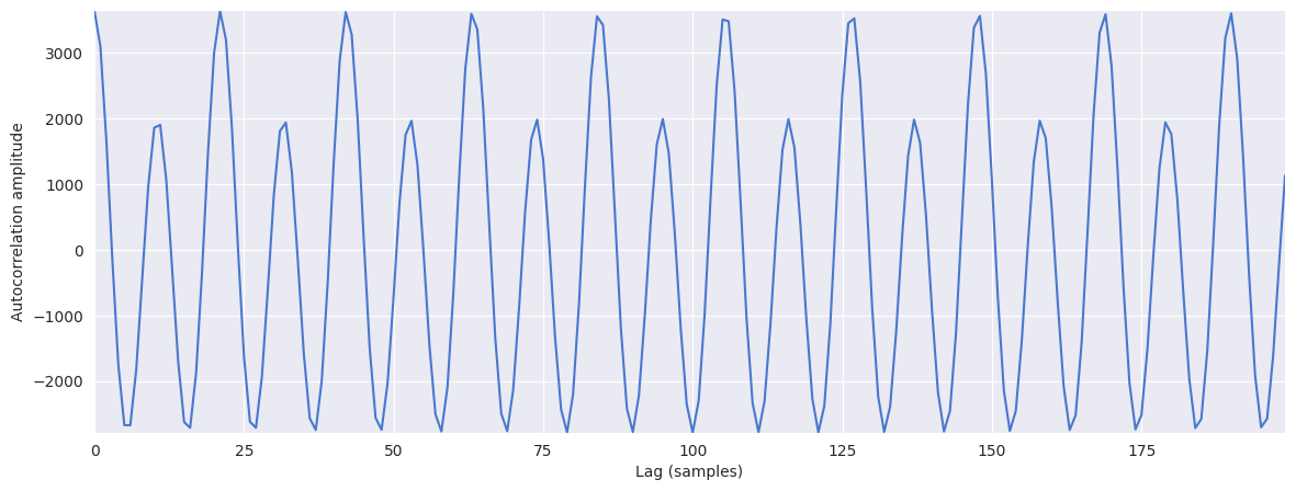
The autocorrelation always has a maximum at zero, i.e. zero lag. We want to identify the maximum outside of the peak centered at zero. Therefore, we might choose only to search within a range of reasonable pitches:

midi_hi = 120.0
midi_lo = 12.0
f_hi = librosa.midi_to_hz(midi_hi)
f_lo = librosa.midi_to_hz(midi_lo)
t_lo = sr / f_hi
t_hi = sr / f_lo

print(f_lo, f_hi)
print(t_lo, t_hi)

16.351597831287414 8372.018089619156
2.633773573344376 1348.4920695523206

Set invalid pitch candidates to zero:

r[: int(t_lo)] = 0
r[int(t_hi) :] = 0

plt.figure(figsize=(14, 5))
plt.plot(r[:1400])
plt.xlabel("Lag (samples)")
plt.ylabel("Autocorrelation amplitude")

Text(0, 0.5, 'Autocorrelation amplitude')

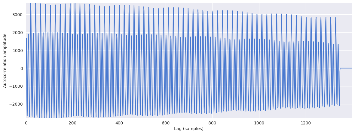
Find the location of the maximum:

t_max = r.argmax()
print(t_max)

21

Finally, estimate the pitch in Hertz:

float(sr) / t_max

1050.0

Indeed, that is very close to the true frequency of C6:

librosa.midi_to_hz(84)

1046.5022612023945

Tempo Estimation

When perfomed upon a novelty function, an autocorrelation can provide some notion of tempo.

For more, see the notebook Tempo Estimation.