Onset-based Segmentation with Backtracking

import IPython.display as ipd
import matplotlib.pyplot as plt
import librosa.display
import numpy

from mirdotcom import mirdotcom

mirdotcom.init()

librosa.onset.onset_detect works by finding peaks in a spectral novelty function. However, these peaks may not actually coincide with the initial rise in energy or how we perceive the beginning of a musical note.

The optional keyword parameter backtrack=True will backtrack from each peak to a preceding local minimum. Backtracking can be useful for finding segmentation points such that the onset occurs shortly after the beginning of the segment. We will use backtrack=True to perform onset-based segmentation of a signal.

Load an audio file into the NumPy array x and sampling rate sr.

filename = mirdotcom.get_audio("classic_rock_beat.wav")
x, sr = librosa.load(filename)
print(x.shape, sr)

(151521,) 22050

Listen:

ipd.Audio(x, rate=sr)

Compute the frame indices for estimated onsets in a signal:

hop_length = 512
onset_frames = librosa.onset.onset_detect(y=x, sr=sr, hop_length=hop_length)
print(onset_frames)  # frame numbers of estimated onsets

[ 20  29  38  57  66  75  84  93 103 112 121 131 140 149 158 167 176 185
 196 204 213 232 241 250 260 269 278 288]

Convert onsets to units of seconds:

onset_times = librosa.frames_to_time(onset_frames, sr=sr, hop_length=hop_length)
print(onset_times)

[0.46439909 0.67337868 0.88235828 1.32353741 1.53251701 1.7414966
 1.95047619 2.15945578 2.39165533 2.60063492 2.80961451 3.04181406
 3.25079365 3.45977324 3.66875283 3.87773243 4.08671202 4.29569161
 4.55111111 4.73687075 4.94585034 5.38702948 5.59600907 5.80498866
 6.03718821 6.2461678  6.45514739 6.68734694]

Convert onsets to units of samples:

onset_samples = librosa.frames_to_samples(onset_frames, hop_length=hop_length)
print(onset_samples)

[ 10240  14848  19456  29184  33792  38400  43008  47616  52736  57344
  61952  67072  71680  76288  80896  85504  90112  94720 100352 104448
 109056 118784 123392 128000 133120 137728 142336 147456]

Plot the onsets on top of a spectrogram of the audio:

S = librosa.stft(x)
logS = librosa.amplitude_to_db(S)
librosa.display.specshow(logS, sr=sr, x_axis="time", y_axis="log")
plt.vlines(onset_times, 0, 10000, color="k")

/tmp/ipykernel_42097/3814083773.py:2: UserWarning: amplitude_to_db was called on complex input so phase information will be discarded. To suppress this warning, call amplitude_to_db(np.abs(S)) instead.
  logS = librosa.amplitude_to_db(S)

<matplotlib.collections.LineCollection at 0x70d23aa79870>

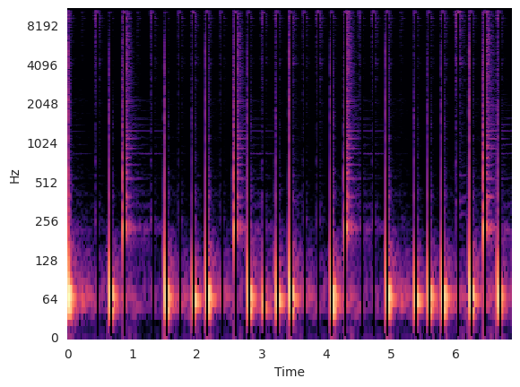
As we see in the spectrogram, the detected onsets seem to occur a bit before the actual rise in energy.

Let’s listen to these segments. We will create a function to do the following:

1. Divide the signal into segments beginning at each detected onset.

2. Pad each segment with 500 ms of silence.

3. Concatenate the padded segments.

def concatenate_segments(x, onset_samples, pad_duration=0.500):
    """Concatenate segments into one signal."""
    silence = numpy.zeros(int(pad_duration * sr))  # silence
    frame_sz = min(numpy.diff(onset_samples))  # every segment has uniform frame size
    return numpy.concatenate(
        [
            numpy.concatenate(
                [x[i : i + frame_sz], silence]
            )  # pad segment with silence
            for i in onset_samples
        ]
    )

Concatenate the segments:

concatenated_signal = concatenate_segments(x, onset_samples, 0.500)

Listen to the concatenated signal:

ipd.Audio(concatenated_signal, rate=sr)

As we hear, the little glitch between segments occurs because the segment boundaries occur during the attack, not before the attack.

Using librosa.onset.onset_backtrack

We can avoid this glitch by backtracking from the detected onsets.

When setting the parameter backtrack=True, librosa.onset.onset_detect will call librosa.onset.onset_backtrack. For each detected onset, librosa.onset.onset_backtrack searches backward for a local minimum.

onset_frames = librosa.onset.onset_detect(
    y=x, sr=sr, hop_length=hop_length, backtrack=True
)

Convert onsets to units of seconds:

onset_times = librosa.frames_to_time(onset_frames, sr=sr, hop_length=hop_length)

Convert onsets to units of samples:

onset_samples = librosa.frames_to_samples(onset_frames, hop_length=hop_length)

Plot the onsets on top of a spectrogram of the audio:

S = librosa.stft(x)
logS = librosa.amplitude_to_db(S)
librosa.display.specshow(logS, sr=sr, x_axis="time", y_axis="log")
plt.vlines(onset_times, 0, 10000, color="k")

/tmp/ipykernel_42097/3814083773.py:2: UserWarning: amplitude_to_db was called on complex input so phase information will be discarded. To suppress this warning, call amplitude_to_db(np.abs(S)) instead.
  logS = librosa.amplitude_to_db(S)

<matplotlib.collections.LineCollection at 0x70d1ff1d5090>

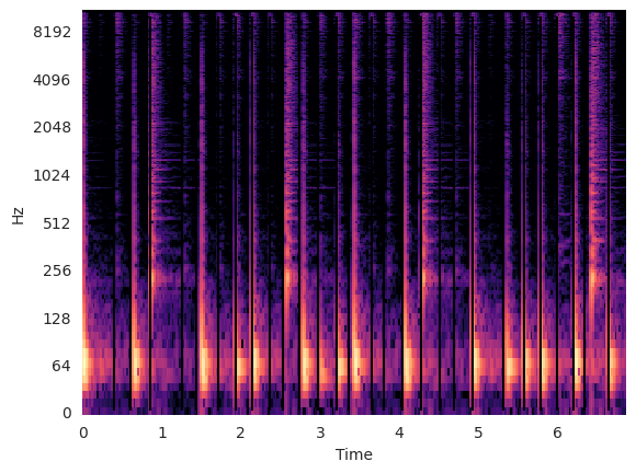
Notice how the vertical lines denoting each segment boundary appears before each rise in energy.

Concatenate the segments:

concatenated_signal = concatenate_segments(x, onset_samples, 0.500)

Listen to the concatenated signal:

ipd.Audio(concatenated_signal, rate=sr)

While listening, notice now the segments are perfectly segmented.

Questions

Try with other audio files:

mirdotcom.list_audio()

simple_piano.wav
latin_groove.mp3
clarinet_c6.wav
cowbell.wav
classic_rock_beat.mp3
oboe_c6.wav
sir_duke_trumpet_fast.mp3
sir_duke_trumpet_slow.mp3
jangle_pop.mp3
125_bounce.wav
brahms_hungarian_dance_5.mp3
58bpm.wav
conga_groove.wav
funk_groove.mp3
tone_440.wav
sir_duke_piano_fast.mp3
thx_original.mp3
simple_loop.wav
classic_rock_beat.wav
c_strum.wav
prelude_cmaj.wav
sir_duke_piano_slow.mp3
busta_rhymes_hits_for_days.mp3